
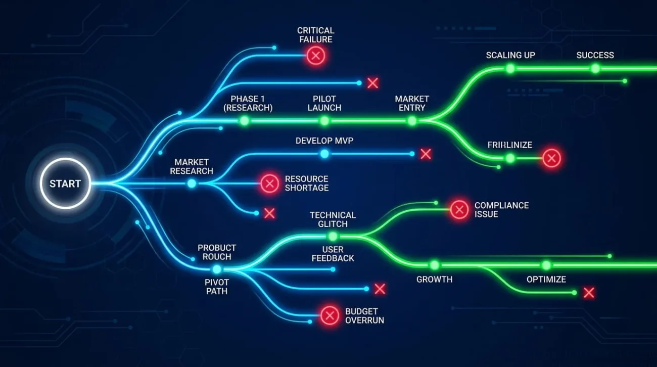
Backtracking is a way to solve problems by building a solution piece by piece. It abandons any partial solution the moment that piece can’t lead to a valid answer. Brute force tests every possible combination. Backtracking checks constraints as it goes and skips entire branches that are already doomed. This single idea, test early and quit early, is what makes backtracking fast enough to solve problems brute force can’t touch.
You’ll find backtracking behind puzzle solvers, route planners, and parsers that compilers use to read code. Say you’ve written a recursive function that tries one choice, calls itself, then undoes that choice before trying the next one. You’ve already written a backtracking algorithm.
The technique matters most on combinatorial problems. Here, the number of raw possibilities grows far faster than any computer could check one by one. Backtracking doesn’t shrink that raw count on paper. In practice, it skips most of it by walking away from dead branches as soon as they appear.
How Backtracking Works
Every backtracking algorithm follows the same rhythm: choose, explore, and unchoose. At each step, the algorithm picks one option from the remaining choices and adds it to the current partial solution. It then checks whether that choice still allows a valid solution. If it does, the algorithm moves forward and repeats the process on the next decision. If it doesn’t, the algorithm removes the last choice and tries a different one instead.
This choose-explore-unchoose pattern is easiest to picture as a tree. Each node represents a partial solution, and each branch represents one possible next choice. Backtracking walks this tree using depth-first search. It moves down a branch as deep as possible before checking whether it needs to climb back up.
Pruning: Why Backtracking Beats Brute Force
Brute-force testing tries every possible combination and checks each one only at the end. That wastes enormous time on combinations that were doomed from the first choice. Backtracking prunes those branches early, the moment a constraint fails, instead of waiting to build the whole candidate first.
In Sudoku, pruning one bad number in the first empty cell can eliminate millions of later combinations before they’re built. That difference is why a well-pruned backtracking solver finishes in milliseconds while a brute force version may never finish at all.
Backtracking vs Brute Force, Recursion, and Dynamic Programming
People often mix up these terms, so here is how they actually differ.
Brute-force checks every possible answer without filtering. Backtracking prunes branches that violate a constraint before they’re fully built. That makes backtracking a smarter, constraint-aware version of brute force rather than a separate family of algorithms.
Recursion is the mechanism, not the strategy. Backtracking is almost always implemented with recursion, since each choice naturally maps to a recursive call. But not every recursive function performs backtracking. A recursive Fibonacci function never undoes a choice, so it isn’t backtracking at all.
Dynamic programming solves problems with overlapping subproblems by storing results and reusing them later. Backtracking usually can’t reuse work this way, because each partial solution is tied to the specific path that produced it. A few problems combine both techniques, but pure backtracking recomputes everything from scratch on each branch.
The General Backtracking Algorithm Template
Most backtracking solutions follow the same basic shape, regardless of the problem they solve:
function solve(candidate):
if candidate is a complete solution:
record candidate
return
for choice in remaining options:
if choice is valid given candidate:
add choice to candidate
solve(candidate)
remove choice from candidate # the “backtrack” step
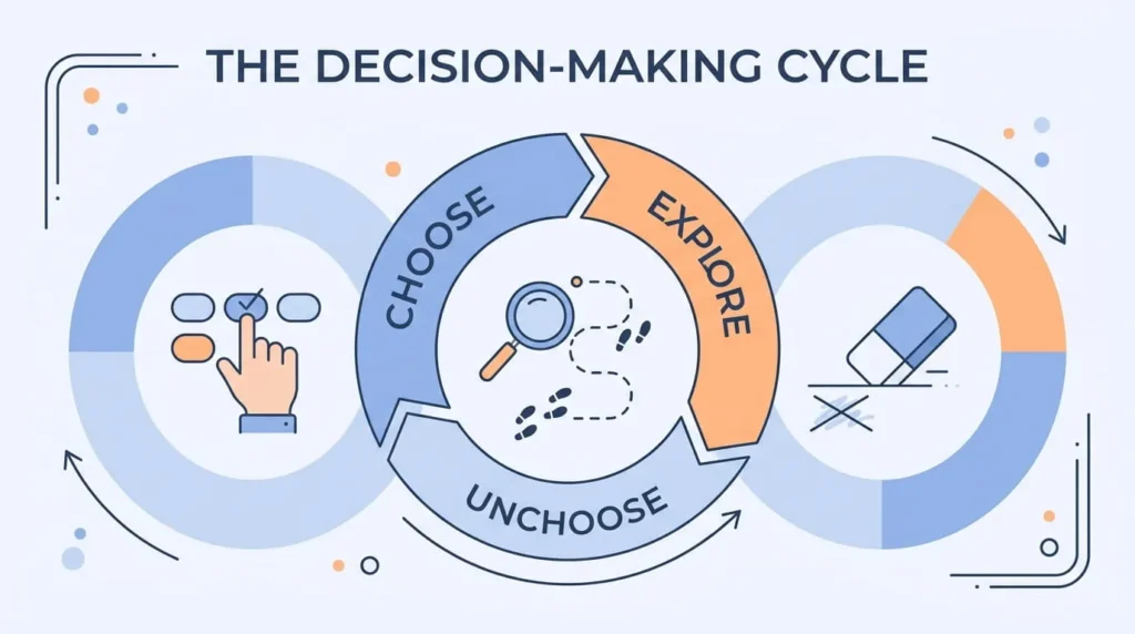
The line that removes the choice after the recursive call is what gives the algorithm its name. Leave that line out, and you have a different search algorithm instead of backtracking.
Classic Backtracking Problems
The N-Queens Problem
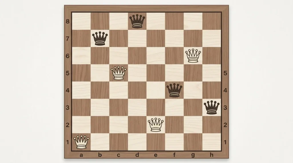
The N-Queens problem asks you to place N chess queens on an N by N board. No two queens can attack each other. Backtracking solves this by placing one queen per row, then checking for a shared column or diagonal with a queen already placed. When a conflict appears, the algorithm removes that queen and tries the next column in that row. This row-by-row placement, combined with early conflict checks, turns billions of raw combinations into a problem modern computers solve almost instantly. That holds at the board sizes used in practice.
Sudoku Solver
A Sudoku solver fills empty cells one at a time, testing digits one through nine in each cell. Before placing a digit, it checks the row, column, and three-by-three box for a conflict. Valid digits get placed, and the algorithm recurses on the next empty cell. Invalid digits get skipped immediately, so the solver never wastes time filling a board already broken by an earlier cell. This constraint check at every single cell is what makes solving even a nearly empty Sudoku grid practical.
Generating Subsets and Permutations
Backtracking generates every subset or permutation of a set one element at a time. For each element, it decides whether to include it or where to place it. For subsets, each element gets an include-or-exclude branch. For permutations, each unused element becomes a candidate for the next position. Both approaches build a result, record it once complete, then undo the last decision before trying the next branch. This is the standard way coding interviews and combinatorics libraries generate every arrangement without missing one or repeating one.
Maze and Pathfinding Problems
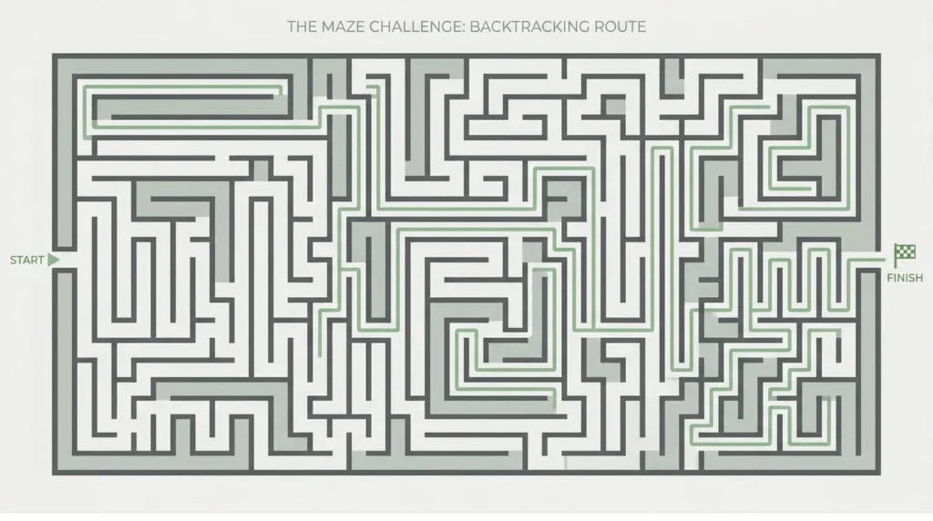
In a maze, backtracking moves one step in a direction, marks that cell as visited, and continues forward. When every direction from a cell is a dead end, the algorithm backs up and tries a different direction. This is why a backtracking maze solver can look like a person feeling their way through a dark hallway. It retreats whenever it hits a wall, rather than mapping the whole maze before taking a single step.
Time Complexity of Backtracking Algorithms
Backtracking algorithms are typically exponential in the worst case, because the number of possible partial solutions grows with every added choice. Consider a problem with b choices at each of d decision points. An unpruned search tree then has roughly b to the power of d leaves.
Good pruning doesn’t change this worst-case bound. It changes actual runtime dramatically by cutting off huge sections of the tree before they’re explored. This is why two backtracking solutions to the same problem can run at wildly different real-world speeds. Both may be exponential in theory. When comparing backtracking approaches, the strength of the pruning condition usually matters more than any other design choice.
The order in which you try choices also affects real-world speed, though it never changes the worst-case bound. Trying the choice most likely to fail first means a bad branch gets cut off after one step instead of ten. On problems like Sudoku or N-Queens, this ordering choice alone can decide whether a solver returns instantly or takes several seconds.
When Backtracking Is the Wrong Tool
Backtracking struggles on problems with heavy overlap between subproblems, since it recomputes the same partial work instead of reusing it. If your backtracking solution keeps rebuilding identical partial states, a dynamic programming approach with memoization will usually run faster.
Backtracking also isn’t a great match for problems where an approximately good answer is enough. Greedy algorithms and heuristic search methods reach a usable answer far faster, even without guaranteeing the best possible one. Reach for backtracking when you need an exact answer and constraints can be checked early. It also fits problems that naturally break into a sequence of choices.
Tips for Writing Efficient Backtracking Code
Check constraints before making a choice, not after building the full candidate, so invalid branches get cut as early as possible.
Order your choices so the option most likely to fail gets tried first, since this prunes bad branches sooner in the search.
Undo every change you make to shared state, arrays, sets, or boards before returning from a recursive call. Otherwise, later branches will see incorrect data.
Stop searching as soon as you have enough solutions. Many problems only need one valid answer or a fixed count, not all of them.
Track visited states with a simple set or boolean grid so the algorithm never explores the same partial solution twice by accident.
Pass the partial solution by reference instead of copying it at every recursive call. Copying a large array or board on each step adds overhead that has nothing to do with the search itself.